patrick@EVERGREEN:~/posts$ cat persistent-kernels.md

Persistent Kernels: Bridging GPU-CPU Execution

contents

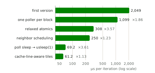
GPUs are fast, but at a cost: launching a kernel costs microseconds on both the host and the device before any computation begins. For the final project of my graduate HPC seminar, I proposed and wrote a persistent kernel (a kernel that is launched once and then runs predefined tasks based on flags in host memory) for an iterative 2D PDE solver on an AMD MI210, to compare it against standard kernel launches. Through multiple optimizations, I improved my persistent kernel from 2,049 µs to 61 µs per iteration, and it beat standard launches at small problem sizes. Looking back on the project now, though, I've found some mistakes, some of which affect the numbers; I cover them in Reflections.

The classic GPU computation paradigm

Although the boundaries are shifting, the GPU (“device”) has classically been treated as an accelerator, while the CPU (“host”) has played the role of orchestrator. To understand why, we consider a datacenter GPU’s architecture: each MI210 contains 104 compute units (CUs), each of which can hold up to 2,048 threads at once.

During execution of a kernel (a GPU program), the GPU spreads a grid of blocks, each up to 1,024 threads, across the CUs, and each block runs entirely on one CU. Within a block, threads are grouped into wavefronts of 64 that execute the same instructions together on different data (SIMD). Every thread in a block shares that CU’s L1 cache and LDS. The L2 cache and the GPU’s main memory are shared by the whole device.

However, this parallelism comes at the cost of setting up a computation on the GPU. First, the workload must be prepared on the host and copied to device memory. Then, the kernel is sent to the GPU; on AMD, the runtime writes a dispatch packet into a queue that the GPU’s command processor watches. The GPU then executes the kernel, which means scheduling, initializing and cleaning up blocks (the kernel may request more blocks than fit on the device at once, or other kernels may compete for them), handling synchronization, and gathering results. Finally, the data must be copied back. Pinned memory and queuing launches back to back hide some of this, but a standard kernel still pays on the order of microseconds of overhead on the device every time it runs. While the asynchronous nature of GPU computation frees up the CPU for other tasks, this overhead can immediately rule out GPUs for latency-sensitive applications such as real-time audio processing or trading.

With these tradeoffs (parallelism vs. overhead), the usual paradigm is for the CPU to hand the GPU large chunks of data-parallel work and collect the results later, while smaller computations stay on the CPU.

Figure 1. Where launch time goes, measured on an NVIDIA V100 by Zhang, Wahib and Matsuoka [1]. A cooperative launch is one where every block the kernel asks for must be resident on the GPU at the same time.

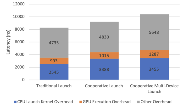
What if this launch and execution overhead didn’t exist?

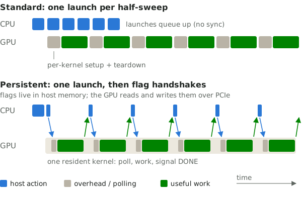
Instead of launching a kernel every time a task needs to run, a persistent kernel runs continuously and communicates with the host to find out which tasks to run and when.I recently came across work that applies the same idea at a much larger scale: Hazy Research’s “megakernel” runs an entire Llama-1B forward pass as one persistent kernel, with an on-GPU instruction interpreter and dependency counters between operations [3].

This approach directly avoids many of the overheads of launching a kernel per task, including the launch and execution overheads. It also allows finer control of the GPU: the programmer decides exactly how blocks or threads are synchronized and how tasks are distributed across blocks.

Figure 2. Standard launches versus a persistent kernel (timeframes not to scale). The persistent kernel trades per-kernel setup for a flag handshake over PCIe.

On the other hand:

• All tasks in one kernel. A persistent kernel cannot be modified once it’s launched, so all the desired tasks have to be implemented together.
• Communication is its own overhead. The host and device poll shared signal variables: the device waits for a signal to start a task, and the host waits for a signal that it’s finished. These signals cost atomics and trips across PCIe.
• The maximum block count is fixed. Unlike a standard kernel, a persistent kernel cannot abstract away the number of blocks. The GPU supports a limited number of blocks per CU (and it has a limited number of CUs).Every block must be resident from launch, because blocks keep running until the kernel terminates; a block that never got scheduled would leave the others spinning forever. I launched the kernel with hipLaunchCooperativeKernel, which only launches if all requested blocks fit on the device.
• Synchronization is the programmer’s responsibility. Combined with everything above, this makes a persistent kernel significantly more difficult to implement than one using the standard launch paradigm.

Sketching out the experiment

For this project, I had two main questions:

1. How do persistent kernels customized for a specific problem perform compared with standard kernels?
2. What is the actual launch and execution overhead of a standard kernel on the problem I chose?

To answer them, I wrote a kernel in each paradigm that solves a computationally intensive iterative problem at various problem sizes. To ensure fairness, I optimized both to the best of my ability, aiming for the point where hardware rather than my implementation was the limit, and I gave both kernels the same block count (up to the point where the device was saturated) so they had identical access to the GPU. After the initial experiments, I further modified the kernels to tease out individual causes of latency.

The problem (another PDE solver)

For the test problem, I adapted a problem from the course: a 2D differential equation solver for Poisson’s equation on the unit square, with corners at \((0, 0)\) and \((1, 1)\),

\[\frac{\partial^2 u}{\partial x^2} + \frac{\partial^2 u}{\partial y^2} = f(x, y).\]

To vary the problem size, I divided each side of the square into \(N\) points, including 0 and 1, which gave an \(N \times N\) matrix \(u\) with spacing \(\Delta = \frac{1}{N-1}\). Approximating both second derivatives with central differences and solving for the center point gives the iterative update rule at a point \(u_{i, j}\):

\[u_{i,j} \leftarrow \frac{1}{4}\left(u_{i+1,j} + u_{i-1,j} + u_{i,j+1} + u_{i,j-1} - \Delta^2 f_{i,j}\right)\]

Derivation

The second-order central difference in each direction is

\[\frac{\partial^2 u}{\partial x^2} \approx \frac{u_{i-1,j} - 2u_{i,j} + u_{i+1,j}}{\Delta^2}, \qquad \frac{\partial^2 u}{\partial y^2} \approx \frac{u_{i,j-1} - 2u_{i,j} + u_{i,j+1}}{\Delta^2}.\]

Adding them and setting the sum equal to \(f(x, y)\):

\[f_{i,j} = \frac{u_{i+1,j} + u_{i-1,j} + u_{i,j+1} + u_{i,j-1} - 4u_{i,j}}{\Delta^2},\]

and solving for \(u_{i,j}\) gives the update above.

I also picked an arbitrary solution, \(u = \sin(2\pi x)\cos(2\pi y)\), which gives \(f(x, y) = -8\pi^2 \sin(2\pi x)\cos(2\pi y)\). After filling in the boundary conditions from that solution (and starting the interior at zero), the iterative solver can run.

Figure 3. Red-black ordering. Each half-sweep updates one color using only neighbors of the other color.

Implementation details and correctness

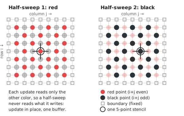
One optimization I used here was to first update every \(u_{i,j}\) where \(i\) and \(j\) have the same parity, then every one where they don’t.This is red-black Gauss-Seidel. Because each update uses newer neighbor values, it converges in about half as many iterations as Jacobi, which computes every point from the previous iteration’s values into a separate result matrix. Along with converging faster, this needs no separate result matrix. A half-sweep never reads a value that the same half-sweep writes, so the update can happen in place. That means less overhead from managing and possibly copying data, so the overhead effects I wanted to examine would be better isolated from confounding factors. For the same reason, I didn’t compute the difference between iterations (to measure convergence) at each time step; those would have required extra synchronizations, and the two kernels would have done those synchronizations differently, which would confound the comparison.I think most production kernels would also skip these synchronizations once testing showed the kernel worked, so I believe this is a valid experimental design choice and doesn’t conflate the research questions.

I ensured correctness and convergence by running a fixed number of iterations and comparing selected elements against a reference implementation that ran the same number of iterations. Due to the iteration logic becoming more complex with red-black and eventually tiling across blocks, I also used a test script to check that the loops covered the whole domain exactly once per iteration. For each optimization and implementation, I ran multiple trials to make sure results were stable and consistent.Looking back on it, this check was too weak: every element I checked was handled by the same wavefront, which hid some errors in my code. More in Reflections.

Optimizing the persistent kernel

In this section, I’ll discuss the optimizations I implemented for the persistent kernel. While optimizing, I used \(N = 1001\) as the problem size, since that was close to the number of blocks the device could hold at once,For the base kernel, that’s 999 blocks at one block per row. The persistent (co-resident) maximum is 104 CUs times blocks per CU; at 256 threads per block, that’s at most 832 blocks (register or LDS usage can lower this, but it didn’t here). and its longer runtimes reduced noise from random variance.

Figure 4. Average time per iteration after each step, at N = 1001 (log scale; ×k is the speedup over the step before). The overall improvement comes out to around 33×. There's a caveat to some of these numbers, which I'll touch on in Reflections.

Base implementation

My naive persistent implementation followed Figure 2. Every thread in every block polled its block’s CPU-to-GPU flag in host memory. When the CPU wrote a task there, the block ACKed it and ran the task (a red or black half-sweep), and then the block’s first thread wrote GPU_DONE to the block’s GPU-to-CPU flag. The CPU waited for every GPU_DONE before sending the next task. All flag accesses were atomics with SEQ_CST memory ordering.

// GPU: every block runs this until it is told to stop
while (true) {
  int signal;
  do {                                   // every thread polls
    signal = atomic_load(&cpu_to_gpu[blockIdx.x]);
  } while (signal == IDLE);
  __syncthreads();
  if (threadIdx.x == 0) atomic_store(&cpu_to_gpu[blockIdx.x], IDLE);
  if (signal == STOP) break;
  run_task(signal);                      // red/black half-sweep
  __syncthreads();
  if (threadIdx.x == 0) atomic_store(&gpu_to_cpu[blockIdx.x], GPU_DONE);
}

// CPU: one half-sweep => signal every block, then wait for all
void half_sweep(int task) {
  for (int b = 0; b < nblocks; ++b)
    atomic_store(&cpu_to_gpu[b], task);
  int pending = nblocks;
  while (pending > 0) {
    for (int b = 0; b < nblocks; ++b)
      if (atomic_load(&gpu_to_cpu[b]) == GPU_DONE) {
        atomic_store(&gpu_to_cpu[b], GPU_WAIT);
        --pending;
      }
    usleep(25);
  }
}
// main: half_sweep(RED); half_sweep(BLACK); ... then STOP

This implementation averaged about 2,049.3 µs per iteration.

Thread synchronization

In my first implementation, I had two calls to __syncthreads(). The first served as a barrier while threads waited for the task signal from the CPU, and the second held threads while they waited to mark the task finished. I later realized this level of synchronization was not needed. Instead of having every thread poll the task flag, I could have one thread poll it and then write the task to a shared variable.Each block has its own shared memory (LDS) on its CU, which is much cheaper to read than host memory over PCIe, especially while polling! At the time, I thought a __threadfence_block() was enough to make sure the shared variable reached the other threads before they used it.A fence only orders the calling thread’s own memory operations. Threads 1–63 still waited for thread 0, but only because they share its wavefront, which is extremely fragile; the other 192 threads in the 256-thread block didn’t wait at all. See Reflections. This also cut the number of atomic calls, which was a big bonus.

int b = blockIdx.x;
if (threadIdx.x == 0) {
  int signal;
  do { signal = atomic_load(&cpu_to_gpu[b], SEQ_CST); }
  while (signal == CPU_WAIT);
  shared_signal = signal;
  atomic_store(&cpu_to_gpu[b], CPU_WAIT, SEQ_CST);
  // early ack, so the CPU can send the next task sooner
  atomic_store(&gpu_to_cpu[b], GPU_DONE, SEQ_CST);
}
__threadfence_block();
switch (shared_signal) { /* red/black half-sweep, or stop */ }

This gave a 1.86× speedup, to an average of 1,099.2 µs per iteration.

Atomics and memory ordering

Something I then noticed was that the device-side atomic loads and stores used the SEQ_CST memory order. At first, I didn’t know what that meant, but while looking for optimizations I realized these operations were quite costly.Why SEQ_CST hurt so much: these atomics are system-scope, since the flags live in host memory. On the MI210 (gfx90a), a system-scope sequentially consistent load makes the compiler emit L2 and L1 cache invalidates after it, and a store emits an L2 write-back [4]. Inside a spin loop, every poll was flushing caches. Since only one thread per block handled communication, I believed ordering didn’t matter beyond the basic guarantees of an atomic variable, so I switched to RELAXED throughout.RELAXED is fine for the flags’ values themselves, but it says nothing about whether the block’s data writes are visible to the neighbors that read them next. See Reflections.

This gave a 3.57× speedup, to an average of 307.7 µs per iteration.

Custom block scheduling

While I was working on the communication protocol, I ran some tests and noticed that some blocks sat idle waiting for others to finish the current task. Some variance in each block’s runtime made sense, so I aimed to reduce the waiting with a more granular scheduling rule for the host-side scheduler: signal each block to execute the next half-sweep as soon as the required data from neighboring blocks is ready, keeping as many tasks in flight as possible.

// host (simplified 1D version): block i may start its next
// half-sweep once neither neighbor is behind it. steps[] counts
// completed half-sweeps; the two edge entries are sentinels.
// This adds no atomics: the host already polls every flag.
if (done[i] && steps[i] <= steps[i - 1] && steps[i] <= steps[i + 1]) {
  int task = (steps[i] % 2 == 0) ? RED_TASK : BLACK_TASK;
  atomic_store(&cpu_to_gpu[i], task, RELAXED);
}

Figure 5. Lockstep (naive) versus neighbor-aware scheduling (simulated durations, for illustration). Blocks can end up several half-sweeps apart, but two neighbors never differ by more than one, so with correct synchronization every block reads the same values it would in lockstep.

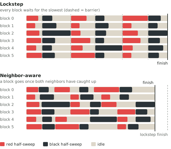
This can leave some blocks further ahead than others, and I worried about numerical instability, but it still converged to very similar results.While reviewing this project, I found that there is actually theory behind this. Chazan and Miranker showed that asynchronous (“chaotic”) relaxation converges for systems like this one as long as staleness is bounded [5]. I’d still want to quantify the effect with full difference calculations.

This gave a 1.23× speedup, to an average of 249.9 µs per iteration.

Tuning sleep duration

This was a simple one. My original sleep durations were now far too long relative to iteration time, so I tested a few values and settled on a single usleep(1) call in the CPU loop.usleep(1) doesn’t sleep for 1 µs. Linux adds a default 50 µs of timer slack to sleeps, so each call is more like 50–60 µs. At smaller sizes, I got the best performance by simply busy-polling.

This gave a 3.61× speedup, to an average of 69.2 µs per iteration.

Cache-line aware tiling and iteration

After a lecture on seismic imaging in class, which emphasized reducing the number of cache lines accessed by a kernel, I tried applying the idea to this problem. Each update reads adjacent cells, so in my naive implementation a block operating on a \(1 \times 999\) row at \(N = 1001\) was touching a \(3 \times 1001\) region, which meant about 189 128-byte cache lines per block per half-sweep. Switching to \(37 \times 27\) tiles shrinks the region each block reads to \(39 \times 29\), and each 29-element row of it spans two or three cache lines, meaning 78 to 117 128-byte cache lines per block per half-sweep.On the MI210, L1 lines are 64 bytes and L2 lines are 128 bytes [2]. I counted in 128-byte lines; a similar result holds for L1 lines.

Figure 6. What each block touches per half-sweep. The tile in B is drawn to scale at the element level.

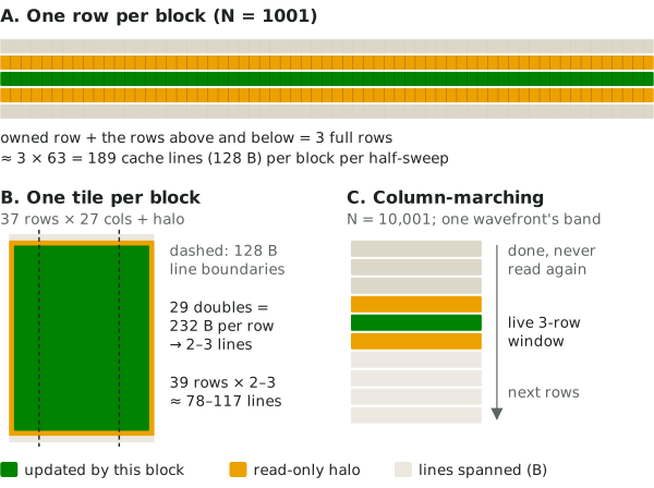
This gave a 1.13× speedup, to an average of 61.22 µs per iteration.

I thought the effect might be more pronounced on a larger problem, so I tried a similar flavor of this optimization at \(N = 10001\) as well. Instead of each block handling a row and then jumping gridDim.x rows ahead to the next one, I had each block handle a band of contiguous rows. And instead of sweeping across those rows one at a time, each thread owned a column and walked down it, so each wavefront swept a 64-column strip downward through the band. At any moment only a three-row window of that strip was live: once the window passed a row, nothing read it again. Going row by row, every pass touched a full 80 KB row, so even though the next pass would need two of those three rows again, by then the small caches had probably evicted them.

At \(N = 10001\), the implementation without this optimization took 3,786.46 µs per iteration; with it, 3,034.42 µs, a 1.25× speedup.

Comparing the kernels

Small problem sizes

The latency effect I was after was supposed to be most significant at small problem sizes (minimal compute), so I tested sizes from \(N = 11\) to \(N = 101\), running 1,000 iterations at each size to reduce noise.

Figure 7. Average time per iteration against problem size. Blue: base kernel, launches queued with no sync (execution overhead). Orange: base kernel with a sync every iteration (adds launch overhead). Green: persistent kernel.

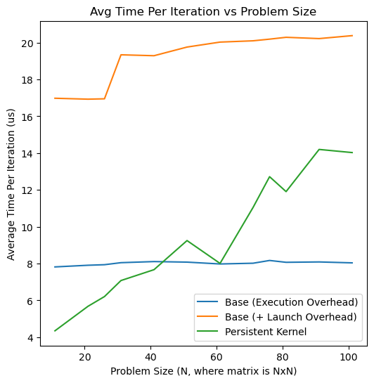
At \(N = 11\) there’s essentially no computation and very little persistent-kernel overhead, so the raw cost of executing a kernel (execution overhead) is shown. The kernel launch overhead itself is mitigated by keeping tasks in flight; red-black allows us to queue tasks without any memory management or synchronization between steps. The gap in average iteration time at \(N = 11\) should therefore mostly be the cost of moving blocks from the queue into execution and shutting them down (about 3–4 µs).That’s per iteration, meaning two half-sweep kernels (red and black), so it’s roughly 2 µs per kernel. Similarly, the persistent kernel’s ~4.3 µs is two handshakes, about 2 µs each, which is roughly one PCIe read round trip plus a write.

To measure the launch overhead, I modified the base implementation to synchronize every iteration. This prevents the mitigation of launch overhead through queued launches. This version is shown in orange, and it suggests the launch overhead is around 10 µs, possibly a bit less once you account for the cost of the synchronize call. This is also closer to what you’d see if you computed a difference at every step, since that needs synchronization too. The slow rise with problem size probably comes from the base kernel launching one block per row. It isn’t host-side: a launch is a single fixed-size dispatch packet no matter how many blocks the grid has. More likely, with a sync every iteration, each kernel’s full duration (including dispatching the extra blocks) is exposed instead of overlapping with the next launch.

At slightly larger sizes, I believe the overhead of managing blocks and doing lots of atomic operations starts to make the persistent kernel slower. My naive block-count rule sets the number of blocks equal to the number of rows and gives each block one row, so this overhead grows linearly with problem size, and that’s what the plot shows. The CPU and GPU poll more and more flags, which means more PCIe traffic and more atomics.The flags are 4-byte ints, packed 16 to a 64-byte host cache line. I didn’t think about cache coherence at the time, but each GPU write invalidates the CPU’s copy of a line that also holds 15 other blocks’ flags. I’d pad the flags so each one gets its own cache line. Going from 9 to 99 blocks adds about 10 µs, or roughly 55 ns per block per handshake, which seems reasonable for a cache miss or two. The base implementation doesn’t pay much more as blocks are added, because the GPU’s hardware dispatcher schedules them in parallel.

Essentially, the results match expectations: at small problem sizes, the persistent kernel wins by eliminating the execution and launch overheads.

Larger problem sizes

Out of curiosity, I also tried larger problem sizes, and got some surprising results. From \(N = 1001\) to \(N = 10001\) the problem gets ~100 times bigger. The persistent kernel went from 61.22 µs to 3,034.42 µs per iteration, an increase of 49.6×, while the base kernel went from 79.9 µs to 9,628.98 µs, an increase of 120.5×. At \(N = 10001\), that made the persistent kernel about 3.2 times faster.

Figure 8. Average time per iteration at larger sizes. The base kernel's time per iteration grew faster than the persistent kernel's.

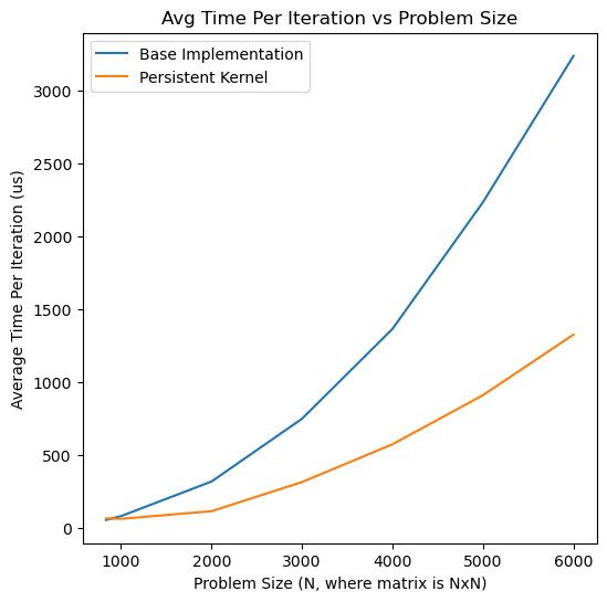
As mentioned earlier, I didn’t apply the cache-line-aware tiling and iteration order to the base kernel the way I did for the persistent kernel. I also didn’t restrict the base kernel to the same number of blocks as the persistent kernel at larger problem sizes, and instead used a block count that made splitting the problem easier. At the time, the persistent kernel’s sublinear growth with problem size looked like the most interesting result. I now think it’s mostly an artifact: there were synchronization errors in this implementation, so the persistent kernel may have been skipping work here (see Reflections).

Roofline

I also plotted both kernels at various problem sizes on the roofline, using the MI210’s 1.6 TB/s peak bandwidth and 22.6 TFLOP/s peak double-precision throughput [2]. As expected, most of these runs are dominated by overhead, so they sit far below both roofs.

Figure 9. Roofline, with every run at the same arithmetic intensity. Small runs are pure overhead.

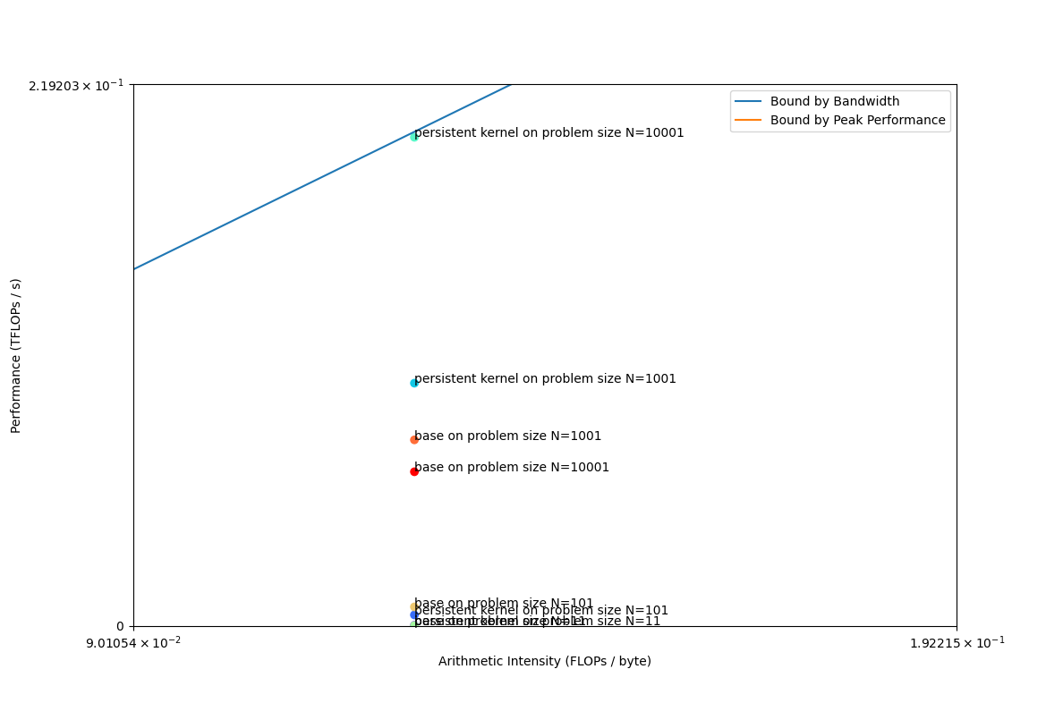
The one interesting point on this plot is the persistent kernel at \(N = 10001\), which sits essentially on the theoretical roof: about 1.58 TB/s of effective bandwidth against a 1.6 TB/s peak. A red-black stencil that uses only half of each cache line it loads shouldn’t get within a few percent of peak bandwidth, so this is a red flag, and it supports the hypothesis that the persistent kernel was skipping work.

Reflections and next steps

As I was reviewing this project, I found a few significant errors and a few points I’d like to improve on, which I’ll discuss here.

1. __threadfence_block() vs. a proper barrier. A fence only prevents reordering of a thread’s own memory operations; a barrier makes other threads wait. A correct implementation would use a barrier after thread 0 publishes the signal, have the other threads acquire-load the shared signal until it changes, or use 64-thread blocks so each block is a single wavefront and no block-wide barrier is needed. (On newer NVIDIA GPUs, lanes of a warp aren’t guaranteed to stay in lockstep, so the single-warp version would still need a __syncwarp() there.) In my implementation, three of the four wavefronts in each block raced ahead, running on stale signals and data, or, if the uninitialized shared signal happened to read as zero, exiting the loop and skipping their share of the work entirely. Thread 0’s wavefront still did its work as intended, but my measured times left out synchronization that should have happened, and possibly work that should have happened too.
2. Memory ordering. RELAXED is enough for the flag values, but it doesn’t guarantee that a neighbor’s halo writes are visible. A correct implementation would spin with relaxed loads, issue an acquire once the signal arrives, and issue a release after the work, before storing GPU_DONE. That would still be much cheaper than system-scope SEQ_CST on every poll, but I’d want to re-run the tests before claiming how much of the 3.57× survives.
3. Early ACKs. My code sent GPU_DONE before the work was done, so the scheduler could start a neighboring block while the halo it reads was only partially updated.
4. Correctness. The check I implemented was too weak: the points it covered all belonged to wavefront 0, so none of these errors got caught. Next time, I’d diff the whole array against the base kernel and make sure there’s no error beyond floating-point tolerance.

Together, these errors could make the solution drift from the correct one, or, if wavefronts exited early, leave parts of the grid never updated. A full diff, which I skipped, would have caught either. Without the first error, asynchronous relaxation would most likely still have converged to the correct solution, just along a different path, since the ordering and early-ACK problems only leave the data a step or two stale. There are also some changes I think would make the comparison fairer:

• Block count differences. At smaller problem sizes, I had too many blocks because I allocated one for each row. That meant more flags for the persistent kernel to poll, and when overhead is the only latency (compute is minimal), it muddies the comparison between kernels. On the other hand, as the problem size increased, I didn’t cap the base kernel’s block count, so the two kernels weren’t splitting the work the same way.
• Cache-line-aware tiling and ordering. I never gave the base kernel the tiling, contiguous row bands, or column-marching iteration order, so the \(N = 10001\) result isn’t fair to it.

I also have a few ideas for making the persistent kernel faster, which is the part of this problem I find most fun:

• GPU-side scheduling. Blocks would spin on their neighbors’ step counters in device memory, taking PCIe out of the loop. This keeps the eager scheduling idea but removes the round trip to the host, and it runs in parallel, while my CPU scheduler is sequential. It’s essentially the dependency-counter approach the megakernel work uses [3].
• Flag padding. Padding the flags to separate cache lines, so one block’s write doesn’t invalidate its neighbors’ flags.
• Better polling. While working on this project, I wasn’t aware of Linux’s timer slack. I’d busy-poll on a pinned core, or shrink the slack with prctl(PR_SET_TIMERSLACK).
• A stronger baseline. HIP graphs let a standard kernel record its whole launch sequence once and replay it, which cuts host-side launch cost. Each kernel still pays its device-side setup, which is exactly the part a persistent kernel avoids, so graphs would be the fairer comparison here.
• Fewer handshakes. With tiles and a wider halo, a block could run several half-sweeps per signal before talking to anyone, trading a little redundant compute at the tile edges for far fewer synchronizations. This would also require maintaining a private working copy of the data in each block, and increase the dependency complexity. An alternative could be each block keeping a 1-wide halo and running multiple steps on its own (on stale data), relying on Chazan-Miranker’s guarantee for convergence. However, this would require more sweeps to converge, and the answer won’t match a strict implementation along the way.

Acknowledgements

Thanks to Dr. Leopold Grinberg (AMD) and to the AMD HPC Fund cluster for access to MI210 GPUs.

References

1. Lingqi Zhang, Mohamed Wahib, and Satoshi Matsuoka. “Understanding the Overheads of Launching CUDA Kernels.” ICPP 2019 (extended abstract).
2. AMD. Instinct MI210 accelerator, and ROCm’s GPU hardware specifications.
3. Benjamin Spector, Jordan Juravsky, et al. “Look Ma, No Bubbles! Designing a Low-Latency Megakernel for Llama-1B.” Hazy Research, 2025.
4. LLVM. AMDGPU Usage: Memory Model GFX90A.
5. D. Chazan and W. Miranker. “Chaotic relaxation.” Linear Algebra and its Applications 2(2), 1969.